LTE uses a linear filter to perform using a set of coefficients like in Equation 1 presented in this paper.

The LTE University.com   quotes the following

“Once the UE is configured to do measurements, the UE starts measuring reference signals from the serving cell and any neighbors it detects. The next question is whether the UE should look at just the current measurement value, or if the recent history of measurements should be considered. LTE, like other wireless technologies, takes the approach of filtering the currently measured value with recent history. Since the UE is doing the measurement, the network conveys the filtering requirements to the UE in an RRC Connection reconfiguration message.”

where

• Mn is the latest received measurement result from the physical layer;
• Fn is the updated filtered measurement result, that is used for evaluation of reporting criteria or for measurement reporting;
• Fn-1 is the old filtered measurement result, where F0 is set to M1 when the first measurement result from the physical layer is received; and
• a = 1 / 2(k/4), where k is the filterCoefficent for the corresponding measurement quantity received by the quantityConfig.

The filterCoefficient is provided to the UE and the sample rate is assumed to be 200ms.

Where is this coming from?

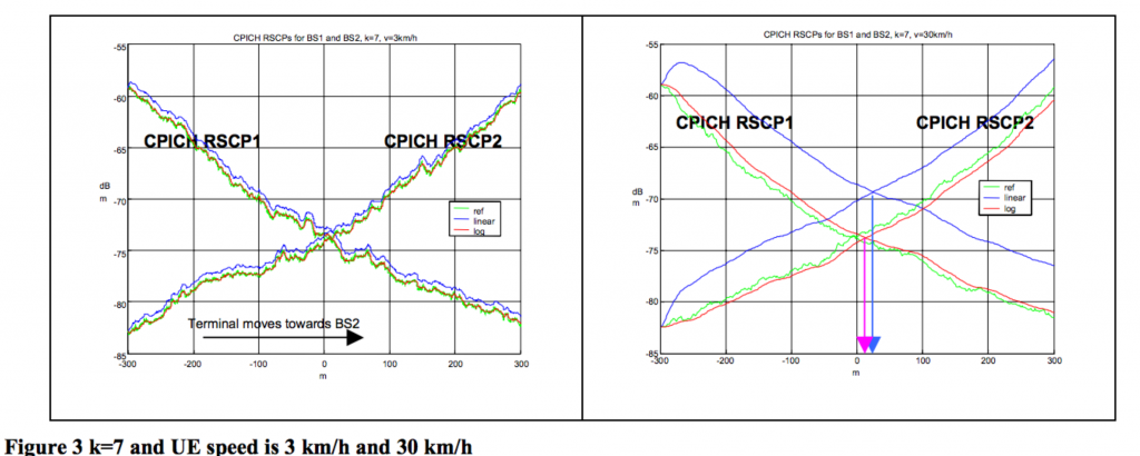
In the following paper, different values of k, and speed are studied to determine which one is the best option to estimate the right value of handover based on previous UE Measurements.

The most interesting conclusion found in this paper is:

” Based on our analyses we can conclude that both of the L3 filters: dB and linear work but they may not have exactly the same performance when a terminal speed varies in a cell. The 3km/h case showed that there is nearly no difference between linear and dB filtering when the length of L3 filtering is such that samples used in L3 filtering are highly correlated. However, in case of higher UE speeds where log-normally distributed fading samples are no longer highly correlated over the whole L3 filtering period difference between linear and dB filtering increases. If we want L3 filtered results (e.g. CPICH RSCP or CPICH Ec/Io results) to follow the actual L1 behaviour better and we want to minimize required soft handover regions in deployments, where L3 filter is used and different terminals may be present in a cell, dB domain L3 filter should be selected. Logarithmic L3 filter also better allows to control the variation of reported absolute CPICH RSCP levels with different speed”

In summary, the use of the proper filtering technique and the right value of speed are keys to minimize required handover regions.  However, the simulation used a PathLoss equation:

PathLoss = 128.1 + 37.6 Log10(R) + LogF

In real life, PathLoss is a function of shadowing, captured by the LogF function.

Another important factor is shown when:

” Figure 3 illustrates well that when terminal speed is relatively small compared to the filter coefficient e.g. 3 km/h for k=7, linear and logarithmic L3 filters do not differ much from each other or from L1 filtered results (the green reference curve). This because the samples used in L3 filtering are highly correlated i.e. variation of different input values to the filters is not high.”

Therefore choosing the right filtering technique will properly anticipate handover with a linear- or log-based filtering.

 

LTE Handover Events

Based on the results of the filtering, several events are triggered in LTE.

A1

Serving becomes better than threshold

A2

Serving becomes worse than threshold

A3

Neighbour becomes offset better than PCell

A4

Neighbour becomes better than threshold

A5

PCell becomes worse than threshold1 and neighbour becomes better than threshold2

A6

Neighbour becomes offset better than SCell

C1

CSI-RS resource becomes better than threshold

C2

CSI-RS resource becomes offset better than reference CSI-RS resource

B1

Inter RAT neighbour becomes better than threshold

B2

PCell becomes worse than threshold1 and inter RAT neighbour becomes better than threshold2

Filtering and Prediction

Linear Prediction Coding is nothing but a linear filter or a low-pass filter.

Wikipedia says that:

Linear prediction is a mathematical operation where future values of a discrete-timesignal are estimated as a linear function of previous samples.In digital signal processing, linear prediction is often called linear predictive coding (LPC) and can thus be viewed as a subset of filter theory. In system analysis (a subfield of mathematics), linear prediction can be viewed as a part of mathematical modelling or optimization.

and Kalman Filter says that:

Kalman filtering, also known as linear quadratic estimation (LQE), is an algorithm that uses a series of measurements observed over time, containing statistical noise and other inaccuracies, and produces estimates of unknown variables that tend to be more accurate than those based on a single measurement alone, by using Bayesian inference and estimating a joint probability distribution over the variables for each timeframe. The filter is named after Rudolf E. Kálmán, one of the primary developers of its theory.

In other words, Filtering is a predictive technique using linear equations that include a Kalman Filter with a linear quadratic estimation .