Predicting Network Traffic using Radial-basis Function Neural Networks – Fractal Behavior
I found a paper about Predicting Network Traffic using RBFNN. I wrote this back in December 2011 regarding Radial-basis Function Neural Networks (RBFNN). Currently, new trends in artificial intelligence are key and RBF-Kernels are in use by machine learning methods and systems.
” Fractal time series can be predicted using radial basis function neural networks (RBFNN). We showed that RBFNN effectively predict the behavior of self-similar patterns for the cases where their degree of self-similarity (H) is close to the unity. In addition, we observed the failure of this method when predicting fractal series when H is 0.5. ”
A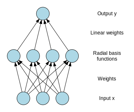 s Hurst-parameter is closer to 0.5 then RBFF are useless to predict fractal behavior, as shown, the randomness of a Hurst parameter at 0.5
For the BRW (brown noise, 1/f²) one gets
- Hq = ½,
and for pink noise (1/f)
Hq = 0.
Obviously, the Hurst Parameter or Hurst Exponent is nothing but a degree of “fractality” for a data set. In General, we don’t expect to predict noise, there is no practical use of for this particular case. we are using the Hurst parameter to see when the RBFF is capable of finding a right response to the data being captured or introduced to the set.
Conclusions
Fractal time series can be predicted using RBFNN when the degree of self-similarity, Hurst parameter, is around 0.9. The mean square error (MSE) of the real and predicted sequences was measured to be 0.36 as a minimum. Meanwhile, fractal series with H=0.5 cannot be predicted as well as the ones with higher values of H.
It was expected that due the clustering process, a better approximation could be achieved using a greater value of M and small dimensionality, however behavior was not observed and in contrast, the performance had and optimal point at M=50 using d=2. This phenomena would require a deeper study and it is out of the scope of this class report.
Future Work
I am retaking this work and combining it with all BigData, this should be co-rrelated with RF and other systems and related research.
Introduction Big Data in RF Analysis | Hadoop: Tutorial and BigData
PREDICTION OF FRACTAL TIME SERIES USING RADIAL BASIS FUNCTION NEURAL NETWORKS
Fractal time series can be predicted using radial basis function neural networks (RBFNN). We showed that RBFNN effectively predict the behavior of self-similar patterns for the cases where their degree of self-similarity (H) is close to the unity. In addition, we observed the failure of this method when predicting fractal series when H is 0.5.
Introduction
We will first review the meaning of the term fractal. The concept of a fractal is most often associated with geometrical objects satisfying two criteria: self -similarity and fractional dimensionality. Self- similarity means that an object is composed of sub-units and sub-sub-units on multiple levels that (statistically) resemble the structure of the whole object. Mathematically, this property should hold on all scales. However, in the real world, there are necessarily lower and upper bounds over which such self-similar behavior applies. The second criterion for a fractal object is that it has a fractional dimension. This requirement distinguishes fractals from Euclidean objects, which have integer dimensions. As a simple example, a solid cube is self-similar since it can be divided into sub-units of 8 smaller solid cubes that resemble the large cube, and so on. However, the cube (despite its self- similarity) is not a fractal because it has an (=3) dimension. [1]
The concept of a fractal structure, which lacks a characteristic length scale, can be extended to the analysis of complex temporal processes. However, a challenge in detecting and quantifying self-similar scaling in complex time series is the following: Although time series are usually plotted on a 2- dimensional surface, a time series actually involves two different physical variables. For example, in Figure 1. the horizontal axis represents “time,” while the vertical axis represents the value of the variable that changes over time. These two axes have independent physical units, minutes and bytes/sec respectively (For example). To determine if a 2-dimensional curve is self-similar, we can do the following test: (i) take a subset of the object and rescale it to the same size of the original object, using the same magnification factor for both its width and height; and then (ii) compare the statistical properties of the rescaled object with the original object. In contrast, to properly compare a subset of a time series with the original data set, we need two magnification factors (along the horizontal and vertical axes), since these two axes represent different physical variables.
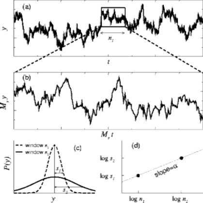 Fig. 1. Fractal time series
In the different windows observed, h1 and h2, we can observe a linear dependency between the variances and windows sizes. In other words, the slope a is determined by (log(s2) – log(s1))/(log(h 1) – log(h2)). This slope value is also called Hurst parameter (H) and in general a value of 0.5 indicates a completely brownian process, whereas 0.99 indicates highly fractal.
The research conducted by Sally Floyd and Vern Paxon [2] concluded that network traffic is fractal in nature and H>0.6. Therefore, RBFNN could be used in this field for network traffic control and analysis. Indeed, we made use of Vern Paxson’s [3,4] method to generate a fractal trace based upon the fractional gaussian noise approximation. The inputs of the Paxson’s program developed are: media, variance, Hurst parameter, and the amound of data. We decided to maintain a media at zero, m = 0, and the variance, σ2=1, and 65536 points. Figures 2 and 3, depict the fractal time series at different sampling windows
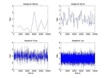
Fig. 2. Fractal sequence sampled at different intervals H=0.5, m =0 and s2 = 1
Fig 2. depicts the generated sampled used for training and testing of the GBRF. The signal is composed of 65536 data samples, ranging between 4 and –4, although we only used 10000 points for training and 10000 points for testing. Similarly, Fig. 3 presents the histogram and fast Fourier transform corresponding to the input in Fig. 2.
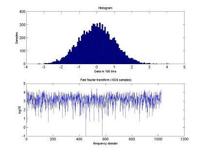
Fig. 3. Histogram and fast Fourier transform of the self-similar sequence H=0.5
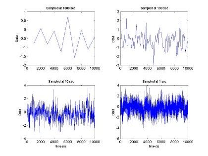
Fig. 4. Fractal sequence sampled at different intervals H=0.9, m =0 and s2= 1
In addition, Fig 4 and Fig 5 show the input data at H=0.9. Both plots show a big difference in the frequency domain among the time series with different values of H. This difference allow us to speculate that RBFNN will be able to perform much better than in the purely random case.
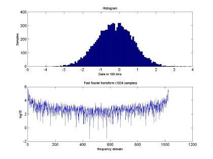
Fig. 5 Histogram and fast Fourier transform of the self-similar sequence H=0.9
Radial basis functions
A radial basis function, like an spherical Gaussian, is a function which is symmetrical about a given mean or center point in a multi-dimensional space [5]. In the Radial Basis Function Neural Network (RBFNN) a number of hidden nodes with radial basis function activation functions are connected in a
feed forward parallel architecture Fig 6.. The parameters associated with the radial basis functions are optimized during training. These parameter values are not necessarily the same throughout the network nor directly related to or constrained by the actual training vectors. When the training vectors are presumed to be accurate ie. Non-stochastic, and it is desirable to perform a smooth interpolation between them, then a linear combination of radial basis functions can be found which gives no error at the training vectors. The method of fitting radial basis functions to data, for function approximation, is closely related to distance-weighted regression. As the RBFNN is a general regression technique it is suitable for both function mapping and pattern recognition problems.
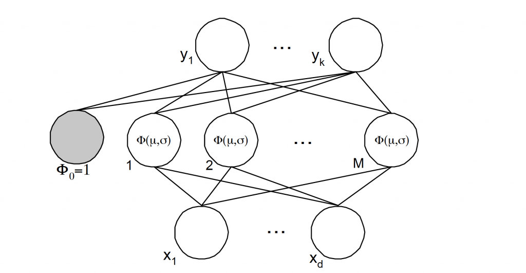
Fig. 6. Radial basis function representation with k-outputs, M-clusters and d-inputs.
The equation required by a Gaussian radial basis function (GRBF) equations are shown as follows:
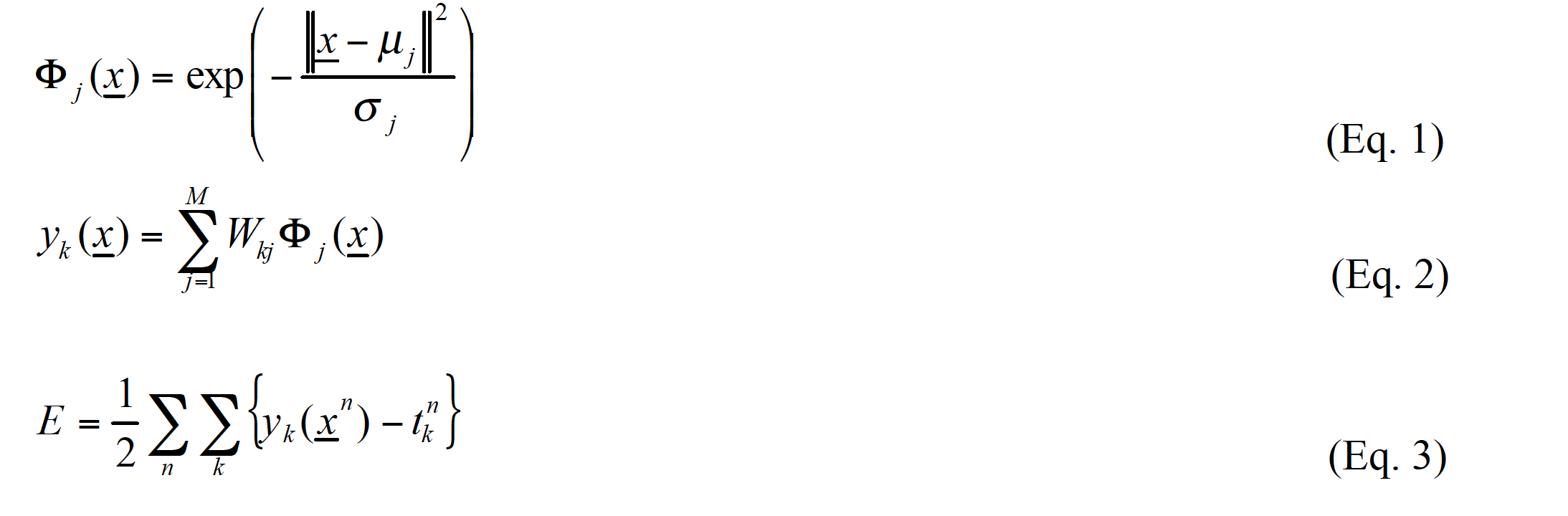
In all cases, n ∈ {1, .. ,N}, or the number of patterns, while k ∈ {1, .., K} or the number of outputs, and j ∈ { 1, .., M} or the number of clusters used on the network.
According to Bishop [6] the solution for the weight matrix is defined as follows:
W T = Φ(Φ)+ T
where all these matrices are defined by:
W = {Wkj }
Φ= {Φ nj }, and Φ nj = Φ j (xn)
T = {Tnk }, Tnk = t nk
And, finally, Y={Ynk }, Y=ΦWT
Therefore, the weight matrix can be calculated with the formula:
WT = Φ +T
Since Φ is a non-squared matrix the pseudo inverse is required to calculate the matrix W.
RBFNN and radial basis functions implemented.
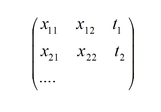
The input to the MATLAB code match up to a file generated by the fractal generator. The set of input data of the fractal file had to be rearranged and organized such that the number of inputs, D, stimulated M- GRBFs. The element D+1 of the sequence was considered as the output. Hence, each sequence of D-inputs will produce one output, which is can be arranged as follows:
{xi }= {{x[n], x[n −1], x[n − 2], x[n − 3],…, x[n − D]}
This set {x i} determines the output tkn , which is x[n+1]. This output is used for training of the RBFNN.
Each term on the {xi} inputs, generates a set of mI and s j input values, where {j ∈ 1..M}, and {i ∈ 1.. N/ (D-1)}. The data is subdivided in N/(MX(D-1)) clusters of D-dimension from which mj and s j are calculated. This calculation was done at the cluster of data by first sorting the data according to tkn or the expected outcome. By sorting the (xn} via tkn we will be able to cluster the input hence each independent basis function will represent a cluster of inputs which can generate a similar outcome.
Hence, it would be expected to have a better predictable value for bigger values of M, or by decreasing the granularity of the cluster. For instance, with d=2, and M=100, given an training set N=3000, we will have a cluster j=1
The cluster of size 10 will have a m1 and m2,, which are the medias of the 10 elements in the first and second columns respectively. The variance is determined using all the elements in the cluster, or both columns are rows. Hence, it would be expected that for a big cluster, or a small value of M and a high- dimensionality this method lead to bigger error during the approximation.
Results and experimental prediction using radial basis functions.
Once the {Φ} matrix is determine, as well as the weight vector W , we proceeded to test the RBFNN with some input data.
Table 1. Variation of M and the mean square error of the training sample at different Hurst parameters
Degree of Self- similarity
|
Hurst Parameter |
|||
|
d-Dimension |
M- GBRFs |
0.9 |
0.5 |
|
2 |
10 |
0.396 |
0.508 |
|
20 |
0.369 |
0.507 |
|
|
50 |
0.349 |
0.514 |
|
|
100 |
0.352 |
0.521 |
|
|
200 |
0.727 |
0.546 |
|
|
4 |
10 |
0.430 |
0.511 |
|
20 |
0.410 |
0.512 |
|
|
50 |
0.380 |
0.523 |
|
|
100 |
0.372 |
0.537 |
|
|
200 |
0.384 |
0.565 |
|
|
8 |
10 |
0.501 |
0.524 |
|
20 |
0.516 |
0.533 |
|
|
50 |
0.466 |
0.566 |
|
|
100 |
0.479 |
0.597 |
|
|
200 |
0.562 |
0.768 |
|
|
16 |
10 |
0.561 |
0.542 |
|
20 |
0.561 |
0.575 |
|
|
50 |
0.676 |
2.735 |
|
|
100 |
4.004 |
29.107 |
|
|
200 |
435.043 |
8.597 |
|
We made use of a sequence, as big as the training input (10000 points). Table 1 depicts the results of the mean square error at different degrees of self-similarity as well as the number of hidden nodes or basis functions used (M).
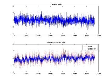
Fig 7. Error and comparison between predicted and real sampled signal for d=2 and M=50. Input signal for H=0.9, 10000 samples used for training
All the input sequences were compared between the original and the predicted input. The best prediction and smaller mean square error (MSE) was observed with d=2, M=50 and H=0.9. This
behavior can be shown also in the qualitative shape shown in Fig. 7. Where the predicted and real sampled data are very similar and the predicted data follows the real sequence. Although the magnitudes are missing, the RBFNN was able to produce a nice input.
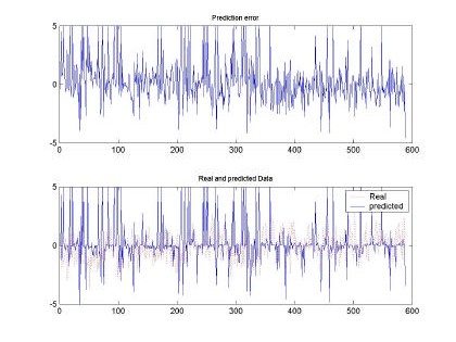
Fig.8 . Error and comparison between predicted and real sampled signal for d=16 and M=200. Input signal for H=0.9, 10000 samples used for training
Meanwhile, Fig. 8, shows the results obtained with H=0.9, M=200, d=16 where we observe that there is
over-estimation on the predicted sequence, which makes the error grow significantly. Those over estimations are not plotted in the figure but rounded between 10 to 20 in magnitude.
Notwithstanding, the MSE seems to grow to unreasonable values, qualitatively the shape of the predicted sequence follows the real testing sample data.
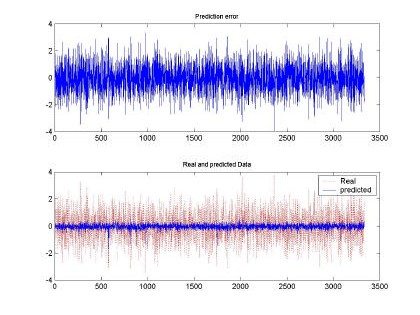
Fig 9. Error and comparison between predicted and real sampled signal for d=2 and M=20. Input signal for H=0.5, 10000 samples used for training
Besides the test executed to the input sequence with H=0.9, Fig. 9 and Fig. 10, depict the behavior of the RBFNN under H=0.5 stimulation. Both plots show the poor performance of the RBFNN when this type of stimulation was employed. In fact, Table 1, presents that the minimum MSE was of 0.5, whereas with H=0.9 the minimum was around 0.3. We have to clarify that for each data set used the RBFNN was trained and its weight matrix calculated using a set of the same input pattern. The performance of the neural network was tested using a training pattern using the same as in the training set.
As show in Fig. 10, the worst performance of the RBFNN was observed when using 16 inputs (d=16) to determine the a predicted pattern and M=100. Although, the error is higher than the MSE measured in Fig 9, qualitatively this shape seems to follow the real sequence used as input.
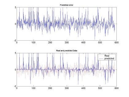
Fig 10. Error and comparison between predicted and real sampled signal for d=16 and M=100. Input signal for H=0.5, 10000 samples used for training
CONCLUSIONS
Fractal time series can be predicted using RBFNN when the degree of self-similarity, Hurst parameter, is around 0.9. The mean square error (MSE) of the real and predicted sequences was measured to be 0.36 as a minimum. Meanwhile, fractal series with H=0.5 cannot be predicted as well as the ones with higher values of H.
It was expected that due the clustering process, a better approximation could be achieved using a greater value of M and small dimensionality, however behavior was not observed and in contrast, the performance had and optimal point at M=50 using d=2. This phenomena would require a deeper study and it is out of the scope of this class report.
APPENDICES
MATLAB CODE USED FOR THE NEURAL NETWORK AND SELF SIMILAR TRACE PRE – PROCESSING
% Fractal sequence processing
% © 2001 – Edwin Hernandez
% selfSimilar = input (‘ Input the name of the file with self-similar
% content ‘);
load selfSimilarH05; x_1 = 1:10;
y_1 = size(10); x_2 = size(100); y_2 = size(100); x_3 = size(1000); y_3 = size(1000); x_4 = size(10000); y_4 = size(10000); j_1=1;
j_2=1; j_3=1; j_4=1;
for i=1:10000,
if (mod(i, 1000) == 0) x_1(j_1) = i;
y_1(j_1) = selfSimilarH05(i); j_1 = j_1 + 1;
end
if (mod(i, 100) == 0) x_2(j_2) = i;
y_2(j_2) = selfSimilarH05(i); j_2 = j_2 + 1;
end
if (mod(i, 10) == 0) x_3(j_3) = i;
y_3(j_3) = selfSimilarH05(i); j_3 = j_3 + 1;
end
x_4(i) = i;
y_4(i) = selfSimilarH05(i); end
subplot(2,2,1); plot(x_1, y_1);
title(‘Sampled at 1000 sec’, ‘FontSize’, 8 );
%xlabel(‘time (s)’,’FontSize’, 8 );
ylabel(‘Data’,’FontSize’, 8 );
subplot(2,2,2); plot(x_2, y_2);
title(‘ Sampled at 100 sec’,’FontSize’, 8 );
%xlabel(‘time (s)’,’FontSize’, 8 );
ylabel(‘Data ‘,’FontSize’, 8 );
subplot(2,2,3); plot(x_3, y_3);
title(‘ Sampled at 10 sec’,’FontSize’, 8 ); xlabel(‘time (s)’,’FontSize’, 8 );
ylabel(‘Data’,’FontSize’, 8 );
subplot(2,2,4); plot(x_4, y_4);
title(‘ Sampled at 1 sec’,’FontSize’, 8 ); xlabel(‘time (s)’,’FontSize’, 8 );
ylabel(‘Data’,’FontSize’, 8 );
pause
subplot(2,1,2), plot(log(abs(fft(y_4, 1024))));
title(‘ Fast fourier transform (1024 samples)’,’FontSize’, 8); ylabel(‘log10’, ‘FontSize’, 8);
xlabel(‘frequency domain’, ‘FontSize’, 8);
subplot(2,1,1), hist(y_4,100); xlabel(‘Data in 100 bins’,’FontSize’,8); ylabel(‘Samples’,’FontSize’, 8);
title(‘ Histogram ‘,’FontSize’, 8);
pause H=20
for i=1:H-1,
x(i) = size(round(10000/H)); end
yk = size(round(10000/5));
% 4 y 1 output to create Yk samples j=1;
load selfSimilarH09; for i=1:H:10000,
for k=0:H-2,
x1(j) = selfSimilarH09(i+k); end
yk(j) = selfSimilarH09(i+k+1); j=j+H;
end
subplot(5,1,1), plot(x1);
subplot(5,1,2), plot(x2);
subplot(5,1,3), plot(x3);
subplot(5,1,4), plot(x4);
subplot(5,1,5), plot(yk);
% Gaussian radial basis functions
% ——————————————————————–
% Edwin Hernandez
% Modified to sort the clusters and then find the Mu’s and the sigmas.
% if M=100 I will sort all the clusters in 100 piles.
D=16;
M=200;
load selfSimilarH09 NDATA = 10000;
% get all the chunks and the T matrix
% out of all the inputs only 65500 I’ll use k=1;
x = size(round(NDATA/(D+1)), D); t = size(round(NDATA/(D+1)));
for j=1:round(NDATA/(D+1)), for i=1:D,
x(j,i) = selfSimilarH09(k);
k=k+1; end k=k+1;
t(j) = selfSimilarH09(k); end
u = size(size(x), D+1); u = [x, t’];
u = sortrows(u, D+1);
x = u(1:size(x), 1:D);
[R,C]=size(x);
t = u(C*R+1:(C+1)*R)’;
%pause;
%cwd = pwd;
%cd(tempdir);
%pack
%cd(cwd)
L = size(t);
cluster = floor(R*C/(M*D)); Mu = size(M, D);
sigma = size(M); Mean = size(D,1); k=0;
for j=1:M,
if (j<M)
z= x(k+1:j*cluster,1:D); k=j*cluster; [l,c]=size(z);
sigma(j) = cov(z(1:l*c)); Mean = mean(z);
%pause; else
z= x(k+1:R,1:D);
k=j*cluster; [l,c]=size(z);
sigma(j) = cov(z(1:l*c));
Mean =mean(z);
end
for i=1:D, Mu(j,i)=Mean(i);
end end
cwd = pwd;
cd(tempdir); pack
cd(cwd)
Phi = size(M, round(NDATA/(D+1))); % M, GBRF ….
for j=1:M,
for k=1:round(NDATA/(D+1)), dist = 0;
for i=1:D,
dist = dist + (x(k, i) – Mu(j, i))^2; end
Phi(j, k) = exp( -2*dist/(2*sigma(j))); end
end
cwd = pwd; cd(tempdir); pack
cd(cwd)
% Weight matrix . W = size(M, 1);
W = pinv(Phi)’*t;
x_test = size(round(NDATA/(D+1)), D); t_test = size(round(NDATA/(D+1)));
k=NDATA+1;
for j=1:round(NDATA/(D+1)), for i=1:D,
x_test(j,i) = selfSimilarH09(k); k=k+1;
end k=k+1;
t_test(j) = selfSimilarH09(k); end
error = size(round(NDATA/(D+1))); y = size(round(NDATA/(D+1))); Phi_out = size(M);
meanSQRerror = 0
for k=1:round(NDATA/(D+1)), for j=1:M,
dist = 0; for i=1:D,
dist = dist + (x_test(k, i) – Mu(j, i))^2; end
Phi_out(j) = exp( -2*dist/(2*sigma(j)));
end
y(k) = Phi_out*W;
error(k) = y(k) – t_test(k);
meanSQRerror = 0.5*(y(k)-t_test(k))^2+meanSQRerror;
if abs(y(k))>=5 y(k) = 5;
end
if abs(error(k))>=5 error(k)=5;
end
end
fprintf(‘The mean square error is : %f’, meanSQRerror); c=round(NDATA/(D+1));
subplot(2,1,1), plot(1:c, error);
title(‘ Prediction error ‘,’FontSize’, 8);
%subplot(3,1,2), hist(error, 100);
%title(‘ Error histogram ‘, ‘FontSize’, 8); subplot(2,1,2), plot(1:c, t_test(1:c), ‘r:’,1:c, y); title(‘ Real and predicted Data ‘, ‘FontSize’, 8); legend(‘Real’,’predicted’);
REFERENCES
- Peng C-K, Hausdorff JM, Goldberger Fractal Analysis Methods http://reylab.bidmc.harvard.edu/tutorial/DFA/node1.html
- Vern Paxson and Sally Floyd, Wide-Area Traffic: The Failure of Poisson Modeling, IEEE/ACM Transactions on Networking, Vol. 3 No. 3, pp. 226-244, June 1995.
- Vern Paxson. Fast Approximation of Self-Similar Network Traffic. Technical Report LBL-36750, Lawrence Berkeley Labs, April 1995.
- Vern Paxson. http://ita.ee.lbl.gov/html/contrib/fft_fgn_c-readme.txt
- Radial Basis Functions. http://www.maths.uwa.edu.au/~rkealley/ann_all/node162.html
- Christopher Bishop “Neural networks for pattern recognition”, Oxford University Press, Birmingham, UK, 1995.